Time collection forecasting with Amazon SageMaker AutoML

Time collection forecasting is a crucial part in varied industries for making knowledgeable choices by predicting future values of time-dependent knowledge. A time collection is a sequence of knowledge factors recorded at common time intervals, akin to each day gross sales income, hourly temperature readings, or weekly inventory market costs. These forecasts are pivotal for anticipating developments and future calls for in areas akin to product demand, monetary markets, vitality consumption, and lots of extra.

Nonetheless, creating correct and dependable forecasts poses important challenges due to elements akin to seasonality, underlying developments, and exterior influences that may dramatically influence the info. Moreover, conventional forecasting fashions typically require intensive area information and guide tuning, which will be time-consuming and sophisticated.

On this weblog put up, we discover a complete method to time collection forecasting utilizing the Amazon SageMaker AutoMLV2 Software program Growth Equipment (SDK). SageMaker AutoMLV2 is a part of the SageMaker Autopilot suite, which automates the end-to-end machine studying workflow from knowledge preparation to mannequin deployment. All through this weblog put up, we will likely be speaking about AutoML to point SageMaker Autopilot APIs, in addition to Amazon SageMaker Canvas AutoML capabilities. We’ll stroll via the info preparation course of, clarify the configuration of the time collection forecasting mannequin, element the inference course of, and spotlight key features of the mission. This technique presents insights into efficient methods for forecasting future knowledge factors in a time collection, utilizing the facility of machine studying with out requiring deep experience in mannequin improvement. The code for this put up will be discovered within the GitHub repo.

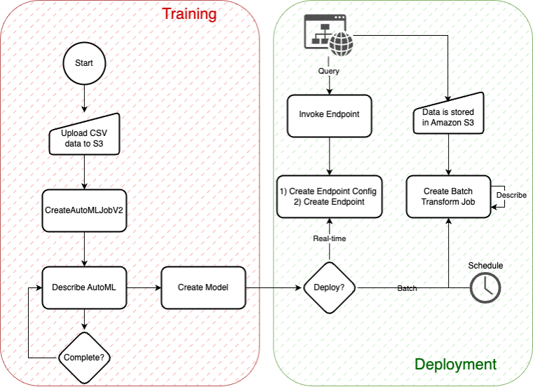
The next diagram depicts the fundamental AutoMLV2 APIs, all of that are related to this put up. The diagram reveals the workflow for constructing and deploying fashions utilizing the AutoMLV2 API. Within the coaching section, CSV knowledge is uploaded to Amazon S3, adopted by the creation of an AutoML job, mannequin creation, and checking for job completion. The deployment section permits you to select between real-time inference through an endpoint or batch inference utilizing a scheduled rework job that shops ends in S3.

1. Information preparation

The inspiration of any machine studying mission is knowledge preparation. For this mission, we used an artificial dataset containing time collection knowledge of product gross sales throughout varied areas, specializing in attributes akin to product code, location code, timestamp, unit gross sales, and promotional info. The dataset will be present in an Amazon-owned, public Amazon Easy Storage Service (Amazon S3) dataset.

When making ready your CSV file for enter right into a SageMaker AutoML time collection forecasting mannequin, you should be certain that it contains no less than three important columns (as described within the SageMaker AutoML V2 documentation):

1. Merchandise identifier attribute title: This column incorporates distinctive identifiers for every merchandise or entity for which predictions are desired. Every identifier distinguishes the person knowledge collection throughout the dataset. For instance, should you’re forecasting gross sales for a number of merchandise, every product would have a singular identifier.
2. Goal attribute title: This column represents the numerical values that you just wish to forecast. These could possibly be gross sales figures, inventory costs, vitality utilization quantities, and so forth. It’s essential that the info on this column is numeric as a result of the forecasting fashions predict quantitative outcomes.
3. Timestamp attribute title: This column signifies the particular occasions when the observations have been recorded. The timestamp is crucial for analyzing the info in a chronological context, which is prime to time collection forecasting. The timestamps needs to be in a constant and applicable format that displays the regularity of your knowledge (for instance, each day or hourly).

All different columns within the dataset are non-compulsory and can be utilized to incorporate further time-series associated info or metadata about every merchandise. Due to this fact, your CSV file ought to have columns named in accordance with the previous attributes (merchandise identifier, goal, and timestamp) in addition to some other columns wanted to help your use case For example, in case your dataset is about forecasting product demand, your CSV would possibly look one thing like this:

• Product_ID (merchandise identifier): Distinctive product identifiers.
• Gross sales (goal): Historic gross sales knowledge to be forecasted.
• Date (timestamp): The dates on which gross sales knowledge was recorded.

The method of splitting the coaching and check knowledge on this mission makes use of a methodical and time-aware method to make sure that the integrity of the time collection knowledge is maintained. Right here’s an in depth overview of the method:

Guaranteeing timestamp integrity

Step one includes changing the timestamp column of the enter dataset to a datetime format utilizing pd.to_datetime. This conversion is essential for sorting the info chronologically in subsequent steps and for making certain that operations on the timestamp column are constant and correct.

Sorting the info

The sorted dataset is crucial for time collection forecasting, as a result of it ensures that knowledge is processed within the appropriate temporal order. The input_data DataFrame is sorted primarily based on three columns: product_code, location_code, and timestamp. This multi-level type ensures that the info is organized first by product and site, after which chronologically inside every product-location grouping. This group is crucial for the logical partitioning of knowledge into coaching and check units primarily based on time.

Splitting into coaching and check units

The splitting mechanism is designed to deal with every mixture of product_code and location_code individually, respecting the distinctive temporal patterns of every product-location pair. For every group:

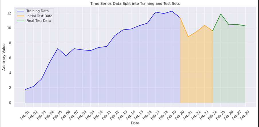
• The preliminary check set is set by choosing the final eight timestamps (yellow + inexperienced beneath). This subset represents the latest knowledge factors which are candidates for testing the mannequin’s forecasting capacity.
• The last check set is refined by eradicating the final 4 timestamps from the preliminary check set, leading to a check dataset that features the 4 timestamps instantly previous the newest knowledge (inexperienced beneath). This technique ensures the check set is consultant of the near-future intervals the mannequin is anticipated to foretell, whereas additionally leaving out the latest knowledge to simulate a practical forecasting situation.
• The coaching set contains the remaining knowledge factors, excluding the final eight timestamps (blue beneath). This ensures the mannequin is skilled on historic knowledge that precedes the check interval, avoiding any knowledge leakage and making certain that the mannequin learns from genuinely previous observations.

This course of is visualized within the following determine with an arbitrary worth on the Y axis and the times of February on the X axis.

The check dataset is used to guage the efficiency of the skilled mannequin and compute varied loss metrics, akin to imply absolute error (MAE) and root-mean-squared error (RMSE). These metrics quantify the mannequin’s accuracy in forecasting the precise values within the check set, offering a transparent indication of the mannequin’s high quality and its capacity to make correct predictions. The analysis course of is detailed within the “Inference: Batch, real-time, and asynchronous” part, the place we talk about the great method to mannequin analysis and conditional mannequin registration primarily based on the computed metrics.

Creating and saving the datasets

After the info for every product-location group is categorized into coaching and check units, the subsets are aggregated into complete coaching and check DataFrames utilizing pd.concat. This aggregation step combines the person DataFrames saved in train_dfs and test_dfs lists into two unified DataFrames:

• train_df for coaching knowledge
• test_df for testing knowledge

Lastly, the DataFrames are saved to CSV information (practice.csv for coaching knowledge and check.csv for check knowledge), making them accessible for mannequin coaching and analysis processes. This saving step not solely facilitates a transparent separation of knowledge for modelling functions but additionally permits reproducibility and sharing of the ready datasets.

Abstract

This knowledge preparation technique meticulously respects the chronological nature of time collection knowledge and ensures that the coaching and check units are appropriately aligned with real-world forecasting situations. By splitting the info primarily based on the final identified timestamps and punctiliously excluding the latest intervals from the coaching set, the method mimics the problem of predicting future values primarily based on previous observations, thereby setting the stage for a strong analysis of the forecasting mannequin’s efficiency.

2. Coaching a mannequin with AutoMLV2

SageMaker AutoMLV2 reduces the assets wanted to coach, tune, and deploy machine studying fashions by automating the heavy lifting concerned in mannequin improvement. It gives a simple method to create high-quality fashions tailor-made to your particular downside kind, be it classification, regression, or forecasting, amongst others. On this part, we delve into the steps to coach a time collection forecasting mannequin with AutoMLV2.

Step 1: Outline the tine collection forecasting configuration

Step one includes defining the issue configuration. This configuration guides AutoMLV2 in understanding the character of your downside and the kind of answer it ought to search, whether or not it includes classification, regression, time-series classification, pc imaginative and prescient, pure language processing, or fine-tuning of huge language fashions. This versatility is essential as a result of it permits AutoMLV2 to adapt its method primarily based on the particular necessities and complexities of the duty at hand. For time collection forecasting, the configuration contains particulars such because the frequency of forecasts, the horizon over which predictions are wanted, and any particular quantiles or probabilistic forecasts. Configuring the AutoMLV2 job for time collection forecasting includes specifying parameters that might finest use the historic gross sales knowledge to foretell future gross sales.

The AutoMLTimeSeriesForecastingConfig is a configuration object within the SageMaker AutoMLV2 SDK designed particularly for organising time collection forecasting duties. Every argument offered to this configuration object tailors the AutoML job to the specifics of your time collection knowledge and the forecasting aims.

time_series_config = AutoMLTimeSeriesForecastingConfig(
    forecast_frequency='W',
    forecast_horizon=4,
    item_identifier_attribute_name="product_code",
    target_attribute_name="unit_sales",
    timestamp_attribute_name="timestamp",
    ...
)

The next is an in depth clarification of every configuration argument utilized in your time collection configuration:

• forecast_frequency
  • Description: Specifies how typically predictions needs to be made.
  • Worth ‘W’: Signifies that forecasts are anticipated on a weekly foundation. The mannequin will likely be skilled to grasp and predict knowledge as a sequence of weekly observations. Legitimate intervals are an integer adopted by Y (12 months), M (month), W (week), D (day), H (hour), and min (minute). For instance, 1D signifies day by day and 15min signifies each quarter-hour. The worth of a frequency should not overlap with the following bigger frequency. For instance, you should use a frequency of 1H as an alternative of 60min.

• forecast_horizon
  • Description: Defines the variety of future time-steps the mannequin ought to predict.
  • Worth 4: The mannequin will forecast 4 time-steps into the long run. Given the weekly frequency, this implies the mannequin will predict the following 4 weeks of knowledge from the final identified knowledge level.

• forecast_quantiles
  • Description: Specifies the quantiles at which to generate probabilistic forecasts.
  • Values [p50,p60,p70,p80,p90]: These quantiles symbolize the fiftieth, sixtieth, seventieth, eightieth, and ninetieth percentiles of the forecast distribution, offering a variety of attainable outcomes and capturing forecast uncertainty. For example, the p50 quantile (median) could be used as a central forecast, whereas the p90 quantile gives a higher-end forecast, the place 90% of the particular knowledge is anticipated to fall beneath the forecast, accounting for potential variability.

• filling
  • Description: Defines how lacking knowledge needs to be dealt with earlier than coaching; specifying filling methods for various situations and columns.
  • Worth filling_config: This needs to be a dictionary detailing easy methods to fill lacking values in your dataset, akin to filling lacking promotional knowledge with zeros or particular columns with predefined values. This ensures the mannequin has a whole dataset to be taught from, bettering its capacity to make correct forecasts.

• item_identifier_attribute_name
  • Description: Specifies the column that uniquely identifies every time collection within the dataset.
  • Worth ’product_code’: This setting signifies that every distinctive product code represents a definite time collection. The mannequin will deal with knowledge for every product code as a separate forecasting downside.

• target_attribute_name
  • Description: The title of the column in your dataset that incorporates the values you wish to predict.
  • Worth unit_sales: Designates the unit_sales column because the goal variable for forecasts, which means the mannequin will likely be skilled to foretell future gross sales figures.

• timestamp_attribute_name
  • Description: The title of the column indicating the time level for every remark.
  • Worth ‘timestamp’: Specifies that the timestamp column incorporates the temporal info essential for modeling the time collection.

• grouping_attribute_names
  • Description: An inventory of column names that, together with the merchandise identifier, can be utilized to create composite keys for forecasting.
  • Worth [‘location_code’]: This setting implies that forecasts will likely be generated for every mixture of product_code and location_code. It permits the mannequin to account for location-specific developments and patterns in gross sales knowledge.

The configuration offered instructs the SageMaker AutoML to coach a mannequin able to weekly gross sales forecasts for every product and site, accounting for uncertainty with quantile forecasts, dealing with lacking knowledge, and recognizing every product-location pair as a singular collection. This detailed setup goals to optimize the forecasting mannequin’s relevance and accuracy to your particular enterprise context and knowledge traits.

Step 2: Initialize the AutoMLV2 job

Subsequent, initialize the AutoMLV2 job by specifying the issue configuration, the AWS position with permissions, the SageMaker session, a base job title for identification, and the output path the place the mannequin artifacts will likely be saved.

automl_sm_job = AutoMLV2(
    problem_config=time_series_config,
    position=position,
    sagemaker_session=sagemaker_session,
    base_job_name="time-series-forecasting-job",
    output_path=f's3://{bucket}/{prefix}/output'
)

Step 3: Match the mannequin

To begin the coaching course of, name the match technique in your AutoMLV2 job object. This technique requires specifying the enter knowledge’s location in Amazon S3 and whether or not SageMaker ought to look forward to the job to finish earlier than continuing additional. Throughout this step, AutoMLV2 will routinely pre-process your knowledge, choose algorithms, practice a number of fashions, and tune them to seek out the most effective answer.

automl_sm_job.match(
    inputs=[AutoMLDataChannel(s3_data_type="S3Prefix", s3_uri=train_uri, channel_type="training")],
    wait=True,
    logs=True
)

Please word that mannequin becoming might take a number of hours, relying on the dimensions of your dataset and compute price range. A bigger compute price range permits for extra highly effective occasion sorts, which might speed up the coaching course of. On this scenario, offered you’re not operating this code as a part of the offered SageMaker pocket book (which handles the order of code cell processing accurately), you have to to implement some customized code that screens the coaching standing earlier than retrieving and deploying the most effective mannequin.

3. Deploying a mannequin with AutoMLV2

Deploying a machine studying mannequin into manufacturing is a crucial step in your machine studying workflow, enabling your purposes to make predictions from new knowledge. SageMaker AutoMLV2 not solely helps construct and tune your fashions but additionally gives a seamless deployment expertise. On this part, we’ll information you thru deploying your finest mannequin from an AutoMLV2 job as a totally managed endpoint in SageMaker.

Step 1: Establish the most effective mannequin and extract title

After your AutoMLV2 job completes, step one within the deployment course of is to establish the most effective performing mannequin, also referred to as the most effective candidate. This may be achieved through the use of the best_candidate technique of your AutoML job object. You possibly can both use this technique instantly after becoming the AutoML job or specify the job title explicitly should you’re working on a beforehand accomplished AutoML job.

# Possibility 1: Straight after becoming the AutoML job
best_candidate = automl_sm_job.best_candidate()

# Possibility 2: Specifying the job title instantly
best_candidate = automl_sm_job.best_candidate(job_name="your-auto-ml-job-name")

best_candidate_name = best_candidate['CandidateName']

Step 2: Create a SageMaker mannequin

Earlier than deploying, create a SageMaker mannequin from the most effective candidate. This mannequin acts as a container for the artifacts and metadata essential to serve predictions. Use the create_model technique of the AutoML job object to finish this step.

endpoint_name = f"ep-{best_candidate_name}-automl-ts"

# Create a SageMaker mannequin from the most effective candidate
automl_sm_model = automl_sm_job.create_model(title=best_candidate_name, candidate=best_candidate)

4. Inference: Batch, real-time, and asynchronous

For deploying the skilled mannequin, we discover batch, real-time, and asynchronous inference strategies to cater to completely different use circumstances.

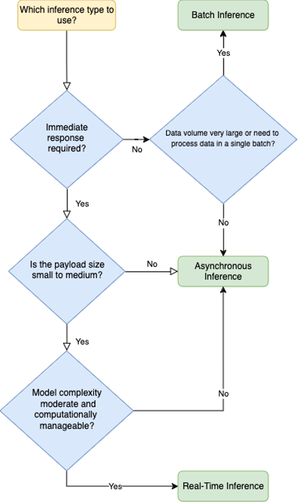
The next determine is a choice tree that can assist you resolve what kind of endpoint to make use of. The diagram outlines a decision-making course of for choosing between batch, asynchronous, or real-time inference endpoints. Beginning with the necessity for quick responses, it guides you thru concerns like the dimensions of the payload and the computational complexity of the mannequin. Relying on these elements, you may select a sooner choice with decrease computational necessities or a slower batch course of for bigger datasets.

Batch inference utilizing SageMaker pipelines

• Utilization: Excellent for producing forecasts in bulk, akin to month-to-month gross sales predictions throughout all merchandise and areas.
• Course of: We used SageMaker’s batch rework characteristic to course of a big dataset of historic gross sales knowledge, outputting forecasts for the required horizon.

The inference pipeline used for batch inference demonstrates a complete method to deploying, evaluating, and conditionally registering a machine studying mannequin for time collection forecasting utilizing SageMaker. This pipeline is structured to make sure a seamless circulation from knowledge preprocessing, via mannequin inference, to post-inference analysis and conditional mannequin registration. Right here’s an in depth breakdown of its building:

• Batch tranform step
  • Transformer Initialization: A Transformer object is created, specifying the mannequin to make use of for batch inference, the compute assets to allocate, and the output path for the outcomes.
  • Remodel step creation: This step invokes the transformer to carry out batch inference on the required enter knowledge. The step is configured to deal with knowledge in CSV format, a standard alternative for structured time collection knowledge.

• Analysis step
  • Processor setup: Initializes an SKLearn processor with the required position, framework model, occasion depend, and sort. This processor is used for the analysis of the mannequin’s efficiency.
  • Analysis processing: Configures the processing step to make use of the SKLearn processor, taking the batch rework output and check knowledge as inputs. The processing script (analysis.py) is specified right here, which can compute analysis metrics primarily based on the mannequin’s predictions and the true labels.
  • Analysis technique: We adopted a complete analysis method, utilizing metrics like imply absolute error (MAE) and root-means squared error (RMSE) to quantify the mannequin’s accuracy and adjusting the forecasting configuration primarily based on these insights.
  • Outputs and property information: The analysis step produces an output file (evaluation_metrics.json) that incorporates the computed metrics. This file is saved in Amazon S3 and registered as a property file for later entry within the pipeline.

• Conditional mannequin registration
  • Mannequin metrics setup: Defines the mannequin metrics to be related to the mannequin bundle, together with statistics and explainability experiences sourced from specified Amazon S3 URIs.
  • Mannequin registration: Prepares for mannequin registration by specifying content material sorts, inference and rework occasion sorts, mannequin bundle group title, approval standing, and mannequin metrics.
  • Conditional registration step: Implements a situation primarily based on the analysis metrics (for instance, MAE). If the situation (for instance, MAE is bigger than or equal to threshold) is met, the mannequin is registered; in any other case, the pipeline concludes with out mannequin registration.

• Pipeline creation and runtime
  • Pipeline definition: Assembles the pipeline by naming it and specifying the sequence of steps to run: batch rework, analysis, and conditional registration.
  • Pipeline upserting and runtime: The pipeline.upsert technique is named to create or replace the pipeline primarily based on the offered definition, and pipeline.begin() runs the pipeline.

The next determine is an instance of the SageMaker Pipeline directed acyclic graph (DAG).

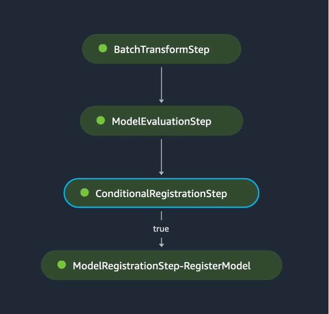
This pipeline successfully integrates a number of phases of the machine studying lifecycle right into a cohesive workflow, showcasing how Amazon SageMaker can be utilized to automate the method of mannequin deployment, analysis, and conditional registration primarily based on efficiency metrics. By encapsulating these steps inside a single pipeline, the method enhances effectivity, ensures consistency in mannequin analysis, and streamlines the mannequin registration course of—all whereas sustaining the pliability to adapt to completely different fashions and analysis standards.

Inferencing with Amazon SageMaker Endpoint in (close to) real-time

However what if you wish to run inference in real-time or asynchronously? SageMaker real-time endpoint inference presents the potential to ship quick predictions from deployed machine studying fashions, essential for situations demanding fast resolution making. When an software sends a request to a SageMaker real-time endpoint, it processes the info in actual time and returns the prediction nearly instantly. This setup is perfect to be used circumstances that require near-instant responses, akin to personalised content material supply, quick fraud detection, and reside anomaly detection.

• Utilization: Fitted to on-demand forecasts, akin to predicting subsequent week’s gross sales for a particular product at a selected location.
• Course of: We deployed the mannequin as a SageMaker endpoint, permitting us to make real-time predictions by sending requests with the required enter knowledge.

Deployment includes specifying the variety of situations and the occasion kind to serve predictions. This step creates an HTTPS endpoint that your purposes can invoke to carry out real-time predictions.

# Deploy the mannequin to a SageMaker endpoint
predictor = automl_sm_model.deploy(initial_instance_count=1, endpoint_name=endpoint_name, instance_type="ml.m5.xlarge")

The deployment course of is asynchronous, and SageMaker takes care of provisioning the mandatory infrastructure, deploying your mannequin, and making certain the endpoint’s availability and scalability. After the mannequin is deployed, your purposes can begin sending prediction requests to the endpoint URL offered by SageMaker.

Whereas real-time inference is appropriate for a lot of use circumstances, there are situations the place a barely relaxed latency requirement will be helpful. SageMaker Asynchronous Inference gives a queue-based system that effectively handles inference requests, scaling assets as wanted to keep up efficiency. This method is especially helpful for purposes that require processing of bigger datasets or advanced fashions, the place the quick response just isn’t as crucial.

• Utilization: Examples embody producing detailed experiences from giant datasets, performing advanced calculations that require important computational time, or processing high-resolution photos or prolonged audio information. This flexibility makes it a complementary choice to real-time inference, particularly for companies that face fluctuating demand and search to keep up a stability between efficiency and value.
• Course of: The method of utilizing asynchronous inference is simple but highly effective. Customers submit their inference requests to a queue, from which SageMaker processes them sequentially. This queue-based system permits SageMaker to effectively handle and scale assets in accordance with the present workload, making certain that every inference request is dealt with as promptly as attainable.

Clear up

To keep away from incurring pointless fees and to tidy up assets after finishing the experiments or operating the demos described on this put up, observe these steps to delete all deployed assets:

1. Delete the SageMaker endpoints: To delete any deployed real-time or asynchronous endpoints, use the SageMaker console or the AWS SDK. This step is essential as endpoints can accrue important fees if left operating.
2. Delete the SageMaker Pipeline: If in case you have arrange a SageMaker Pipeline, delete it to make sure that there aren’t any residual executions which may incur prices.
3. Delete S3 artifacts: Take away all artifacts saved in your S3 buckets that have been used for coaching, storing mannequin artifacts, or logging. Make sure you delete solely the assets associated to this mission to keep away from knowledge loss.
4. Clear up any further assets: Relying in your particular implementation and extra setup modifications, there could also be different assets to think about, akin to roles or logs. Examine your AWS Administration Console for any assets that have been created and delete them if they’re not wanted.

Conclusion

This put up illustrates the effectiveness of Amazon SageMaker AutoMLV2 for time collection forecasting. By rigorously making ready the info, thoughtfully configuring the mannequin, and utilizing each batch and real-time inference, we demonstrated a strong methodology for predicting future gross sales. This method not solely saves time and assets but additionally empowers companies to make data-driven choices with confidence.

In case you’re impressed by the probabilities of time collection forecasting and wish to experiment additional, think about exploring the SageMaker Canvas UI. SageMaker Canvas gives a user-friendly interface that simplifies the method of constructing and deploying machine studying fashions, even should you don’t have intensive coding expertise.

Go to the SageMaker Canvas web page to be taught extra about its capabilities and the way it might help you streamline your forecasting tasks. Start your journey in the direction of extra intuitive and accessible machine studying options at present!

In regards to the Authors

Nick McCarthy is a Senior Machine Studying Engineer at AWS, primarily based in London. He has labored with AWS shoppers throughout varied industries together with healthcare, finance, sports activities, telecoms and vitality to speed up their enterprise outcomes via the usage of AI/ML. Outdoors of labor he likes to spend time travelling, making an attempt new cuisines and studying about science and expertise. Nick has a Bachelors diploma in Astrophysics and a Masters diploma in Machine Studying.

Davide Gallitelli is a Senior Specialist Options Architect for AI/ML within the EMEA area. He’s primarily based in Brussels and works carefully with prospects all through Benelux. He has been a developer since he was very younger, beginning to code on the age of seven. He began studying AI/ML at college, and has fallen in love with it since then.